How monetr's similar transactions work

One of the coolest problems that I was able to work on with monetr was trying to come up with a way to group transactions together. I wanted to be able to view a transaction and in the same view see other similar transactions. This simple idea has a lot of things that can be built on top of it. Similar transactions will have patterns, like recurring dates, or amounts that vary seasonally. I can surface data to the user about these patterns and even use some of them to automate parts of setting up a user’s budget. At least that’s the long term idea.

But getting there the first problem is “group similar transactions”. Initially I explored simply comparing every transaction to every other transaction using Levenshtein Distance with the names or memo of the transaction. This was extremely computationally expensive and even for a dataset of around 1000 transactions was very slow. It also didn’t handle nuances very well since the value or meaningfulness of each word in a transactions memo was the same. Two transactions for different merchants but with slightly similar spelling could be considered the same. The false positive rate seemed very high even just testing this against my own transaction data.

Eventually I found tf-idf, or “term frequency-inverse document frequency”. This algorithm measures the frequency of words in a set of documents (transactions in this case) and gives each word a value that intends to represent how significant that word is in that document. Words that appear in every document are given less value overall, and words appearing in fewer documents are given more value. Words that appear more often in a single document are also considered more valuable within that document, but this is weighted against how often that word appears in all of the other documents.

Here is an example of a transaction name or memo that I’m dealing with in my own dataset:

POS DEBIT-DC 1234 TST* CARIBOU COFFE NORTH BRANCH MN

Most of the transactions in my dataset follow this format. The first word is the payment method, in this case POS or “Point of Sale”. Other transactions may have other payment methods like ACH though. Then the direction of the payment, DEBIT in this case. The last 4 of my card number. Then the actual merchant information, and in this case the town that the merchant is located in.

An assumption I made is that not all of the transaction data that monetr deals with will follow this same pattern. But that generally, within a single institution (your own bank); transactions would follow a consistent format. Even if the order of the data changed, a bank will always have these pieces of information in some form in the memo of their transaction. The words they use might change as well, maybe WITHDRAWAL instead of DEBIT. But as long as every transaction from that bank used the same pattern, it shouldn’t matter.

That assumption plays into how I ended up using tf-idf, and how tf-idf ultimately ended up being the solution. There are shortfalls here that I’ll address later on, but the premise of this is basically: All transactions from an institution will follow a consistent pattern, so meaningless words such as “debit”, “pos”, “transfer” or things that appear in almost every transaction are easy to assign a low value using tf-idf. With that, the more meaningful parts of a transaction will naturally become more valuable. Not every transaction will contain the words CARIBOU COFFE, so those words will be more significant.

The way this works in monetr is a transaction memo such as the one above is taken and “tokenized”. The result of that tokenization looks like this:

First it takes all of the known good words out of the text. This step can sometimes omit specific words that are simply known to be useless, such as null or inc.

POS DEBIT-DC 1234 TST* CARIBOU COFFE NORTH BRANCH MN

Then it transforms them all to be cased consistently and removes unnecessary text. This step also might apply some basic spelling corrections, such as adjusting coffe to be coffee.

pos debit caribou coffee north branch

Overall this is what is happening:

1. Split the string by non-word characters.
2. Throw out any words that are purely numeric or contain no vowels, these are usually pieces of information that are not valuable anyway.
3. Throw out any words from a “drop word” lookup table, this table (as mentioned above) removes words that are universally considered low value regardless of context. Such as null or inc.
4. Throw out any words from a state lookup table, this lookup table will remove words that are in a list of state 2 letter characters. So CA or NY is thrown out.
5. Correct any words using a lookup table, some basic spelling things can be corrected here as sometimes words are truncated. COFFE becomes Coffee.
6. Store a copy of all of the words in lower case so that our tf-idf is not case sensitive.

These transformations give us an array of words or “tokens” that can now be fed into our tf-idf algorithm.

tf-idf

Now that the data has been transformed into a useful format, the data is fed into the tf-idf algorithm. For every transaction (or document) each word is taken and added to a “word count” map that is specific to that document. Then the term frequency of each word is calculated. Taking the number of times that specific word is seen in the document divided by the number of words in the document. This term frequency is then stored for later use. We also increment the global counts for each word.

Once all of the documents have been added, the “idf” can be calculated. This is done using the following formula.

Now we have an individual document frequency for every word among all of our transactions. This on its own is valuable in that it will already show which words show up in almost every transaction.

Then for each document monetr will calculate two parts. The first part is the final tf-idf for that specific document as well as a “vector” which monetr uses for the next stage. The tf-idf is per word, so for every word in a single document we look up what the idf of that word is that we calculated above and we multiply it by the term frequency inside that specific document:

Now monetr knows how much each word in each transaction is “worth” and it needs to turn this data into a way of finding similar transactions. Simply, we can take all of these values of all of these words and assign each unique word a position in a vector. Words that are more significant will have a higher value in the vector and words that are less significant will have a lower value. Words that aren’t present in that specific document will have a value of 0 in this vector.

To make this easy monetr takes all of the words observed in all of the transactions and sorts them alphabetically. Then creates a vector that is the at least the length equal to the number of words seen but rounded up to the nearest size that is divisible by 16.

The reason we round up to 16 is so that the vector fits nicely into SIMD registers used for our normalization and distance functions. On computers that support X86’s AVX instructions these registers allow us to work with 8 values from the vector at a time (using a 256-bit register), on newer hardware that supports AVX512 we can work with 16 values at a time (using a 512-bit register). Keeping the vector a size that is divisible by 16 means that we never need to worry about aligning memory for these operations or handling tailing values of odd sizes. Which keeps the assembly code much simpler and doesn’t require branching logic outside of iterating over the vector.

All in all, by the end of this initial tf-idf process we get a vector of 32-bit floats that looks like this for a given transaction:

vector := []float32{
  0.000000, // acctverify
  0.000000, // ach
  0.000000, // adjustment
  // ...
  0.293779, // branch
  // ...
  0.340398, // caribou
  // ...
  0.339518, // coffee
  // ...
  0.014512, // debit
  // ...
  0.294113, // north
  // ...
  0.045037, // pos
  // ...
  0.000000, // withdrawal
  0.000000, // xfer
  0.000000, //
}

Notice that the only words with a non-zero value in our vector are the words that were in our tokenized transaction string. Each of these words now serves as it’s own “dimension” within the vector, with absent words having no value. But words that are present in our transaction have not only a non-zero value, but also have a higher value if that particular word is considered more “meaningful” relative to the rest of the dataset. This can be seen with the words caribou and coffee having higher values than words that appear more frequently in all other documents such as pos and debit. Also note the padding at the end, even though these values are 0.000000 I included it above to show how the vector is padded to the nearest value divisible by 16 (the example is not showing the value for every single word).

Once we have this vector built we modify the vector using Euclidean normalization¹. We do this to make the data behave more sanely when it comes to the following DBSCAN algorithm that will be discussed below.

To begin, we represent our vector above as $\mathbf{x}$:

Given the vector above where $n$ is divisible by 16, we can use SIMD for the following operations. Create a sum of the squared values of the vector and calculate it’s square root. This is our “norm” that we’ll use below.

Then change the original vector, dividing each value by the “norm” we derived from above.

This normalization makes the vector more uniform while preserving the ratios between the values within that vector. For example, consider the original vector above. The result after normalization would be:

vector := []float32{
  0.000000, // acctverify
  0.000000, // ach
  0.000000, // adjustment
  // ...
  0.460952, // branch
  // ...
  0.534099, // caribou
  // ...
  0.532719, // coffee
  // ...
  0.022770, // debit
  // ...
  0.461476, // north
  // ...
  0.070664, // pos
  // ...
  0.000000, // withdrawal
  0.000000, // xfer
  0.000000, //
}

This process is repeated for every transaction within a single bank account in monetr, resulting in an array of vectors that can now be compared with the next step in the process.

DBSCAN

At this point monetr has an array of vectors with each vector representing what is “meaningful” about the associated transaction. This data can now be used to determine which transactions are similar to each other. To do that monetr uses an algorithm called DBSCAN and Euclidean Distance as the distance function.

The way DBSCAN works is it iterates over all of the data procedurally. It takes the first vector and looks for other vectors in the dataset that are “neighbors”. Vectors within a certain euclidean distance of the initial vector. If it finds at least a minimum number of neighbors within that distance, then that is considered the “root” of a cluster. If it does not find the minimum number of neighbors though, then that means that there are no other transactions that are “similar” to that initial one (or at the very least, that there are not a sufficient number of transactions for this transaction to be considered part of a group of similar transactions). That transaction is marked as “noise” or “visited” so that it is excluded from future calculations.

But transactions that do have neighbors get built out even more. Each of the neighbors are then addressed recursively, looking for each of their neighbors. This allows the cluster of similar transactions to expand as long as there are vectors within the distance threshold specified. This process is repeated until the cluster cannot expand anymore.

Because each word in our dataset is given a specific index in our vector, each word represents a dimension for every transaction. Words that aren’t present in that transaction have no value in that dimension. If there were only 3 words in the dataset then you could express the similarity of transactions with X, Y and Z coordinates. If a transaction contains the word for the X coordinate, then that transaction is pushed out in 3D space on that coordinate. But if the transaction also contains the word for the Y coordinate, then it is also pushed out on the Y coordinate. This results in each transaction having some location within this 3D space, and all DBSCAN is doing is looking for clusters of these coordinates that are close together. Transactions might share the same word but words that are more valuable will have more influence on the coordinates of the transaction, and transactions that share words that are valuable will have coordinates that are proximate in this highly dimensional space.

The result of all of this is that we now have an array of clusters of transactions. We know that within each cluster the transactions therein are at least somewhat similar. The similarity however is not perfect, as I’ll cover below.

Consistently identifying clusters

The next important part of this process is being able to consistently identify the clusters, this way as transactions are added and clusters grow we can still know that it is the same cluster over time. This is not as simple as selecting a transaction ID from the cluster and deciding that it is the “basis” of a cluster and using it as the unique identifier. The cluster could be built poorly initially when there is not sufficient data, but then changes as more data makes the similarities more accurate. This ID would stay the same but the members of the cluster will have changed.

To do this, monetr takes all of the vectors from a similar transaction cluster and tries to calculate which one of the vectors is the center-most or centroid of the cluster. Given that it is likely that many of the transactions may have identical transaction names used for this calculation, there may be multiple transactions that meet this “center-most” criteria. If that is the case, we use the transaction with the lowest ID alphabetically as our centroid or base transaction.

From this we take all of the words that appear in the centroid transaction and sort them by their value. The most valuable words for a transaction rise to the top here. For example, a cluster of transactions for the Caribou Coffee transaction above would have the most valuable words like this:

[
  {
    "word": "Caribou",
    "sanitized": "caribou",
    "order": 4,
    "value": 151.68399,
    "rank": 0.5677639
  },
  {
    "word": "Coffee",
    "sanitized": "coffee",
    "order": 5,
    "value": 151.29242,
    "rank": 0.5648364
  },
  {
    "word": "North",
    "sanitized": "north",
    "order": 6,
    "value": 131.05951,
    "rank": 0.42386284
  },
  {
    "word": "Branch",
    "sanitized": "branch",
    "order": 7,
    "value": 130.91055,
    "rank": 0.42289993
  },
  {
    "word": "Pos",
    "sanitized": "pos",
    "order": 0,
    "value": 20.068632,
    "rank": 0.009938569
  },
  {
    "word": "Debit",
    "sanitized": "debit",
    "order": 1,
    "value": 6.466796,
    "rank": 0.001031969
  }
]

In the example above, the value field is the sum of all of the tf-idf values for that word in each individual transaction in the similar transaction cluster. The rank is the value divided by the number of transactions in the cluster to try to create an average. This helps smooth out any outliers where maybe a few transactions within a cluster have a word that is considered very valuable or meaningful, but might not be present or is considered less valuable in the other transactions in the same cluster.

You can see that the value of the two meaningful words is much higher than the less meaningful words (the location of the transaction). We then take the top 75% of ranked words within this list and we sort them by the order they appeared in the transaction (because the order of the words is not represented by their value necessarily).

[
    {
      "word": "Caribou",
      "sanitized": "caribou",
      "order": 4,
      "value": 151.68399,
      "rank": 0.5677639
    },
    {
      "word": "Coffee",
      "sanitized": "coffee",
      "order": 5,
      "value": 151.29242,
      "rank": 0.5648364
    }
  ]

So for our example, our transaction cluster would be given the name Caribou Coffee. As these are the most valuable words in that cluster.

Caribou Coffee

This ends up being a pretty reasonable way to derive a merchant name from a transaction without the data being sanitized for us already (something that Plaid offers). So this can be used as a way to enrich offline data that is provided via file imports or less reliable data connectors in the future.

But the values of these words might change over time so we still need a good way to identify the cluster consistently as new transactions appear. To do this we make the assumption that the order of the most valuable words may change in the future, maybe coffee becomes more valuable that caribou as an example. But we assume that those words (and the most valuable words in any cluster) will remain within our upper 75% threshold consistently over time.

So to create an identity for this cluster, we’ll take these most valuable words and we’ll sort them alphabetically, convert them to lowercase and then simply SHA256 hash them. This way clusters that share the same signature can also be merged meaningfully, but it also means that we can lookup this signature in the database when we append or modify transaction clusters in the future².

Room for improvement

This entire process is very much “good enough”³, my goal was to build something that provided similar transactions in a way that did not rely on the use of AI models that were difficult to scrutinize. Or in a way that required huge sets of training data to get just right. The assumptions I made here about how transaction data exists is very much “good enough”³. However with that there are some huge spaces for improvement.

1. There are too many dimensions, there is one dimension per word for the entire transaction dataset. While this might not necessarily diminish the “accuracy” of the process on its own, it makes the process significantly less efficient. Most vectors that are compared in the DBSCAN process are primarily 0.0 values, with the exception of maybe 2-6 non-zero values. This means that a lot of the “optimized” assembly code I’ve written is computing nothing most of the time. There are some safe assumptions I could make to improve this. Right now the values are only ever positive, but they don’t need to be. For example, I could combine two words into a single dimension as long as those two words never appear on the same transaction. A negative value on that dimension would represent one word, and a positive value would represent another word. This would reduce the size of the vector (potentially significantly) without any loss in the quality of the output.
2. Words are not exactly the greatest things to index on and some words can be shared between irrelevant transactions. For example, if you have a transaction POS DEBIT-DC 1234 WHITE CASTLE 0800 FOREST LAKE MN and a transaction POS DEBIT-DC 1234 TST* CARIBOU COFFE WHITE BEAR LA MN. The tf-idf process has no way of distinguishing the WHITE in the first transaction from the WHITE in the second transaction. This can skew transaction similarity and cause some weird issues where some words that are meaningful are not treated as such because of how common the word is. The way I would try to solve this is by instead calculating the tf-idf values of word pairs. For example ["pos debit", "debit white", "white castle", "castle forest", "forest lake"]. This rolling pairwise tokenization would allow for better values of pairs of words that are significant. However this essentially ruins any concept of “document frequency” because a “word” (word pair) won’t really ever appear in a document twice. So I would still need to take into consideration individual words somehow.
3. Right now this entire process is re-performed from scratch every time there are transaction changes (file upload or Plaid webhook). This is not efficient at all and while the entire process is pretty quick (a few seconds even for huge accounts) it could be improved significantly if I could capture parts of the data and cache it or store it somewhere and only recalculate what was needed. I have some ideas here but want to get the output really refined first.
   • It is worth noting here that the DBSCAN portion of this is the most expensive part of this by far. Calculating the tf-idf for every transaction (including querying the database for every transaction for a specific bank account) is essentially negligible compared to how long the DBSCAN can take. This can be seen in the screenshot below which is a trace from a production account calculating similar transactions after having received a Plaid webhook. 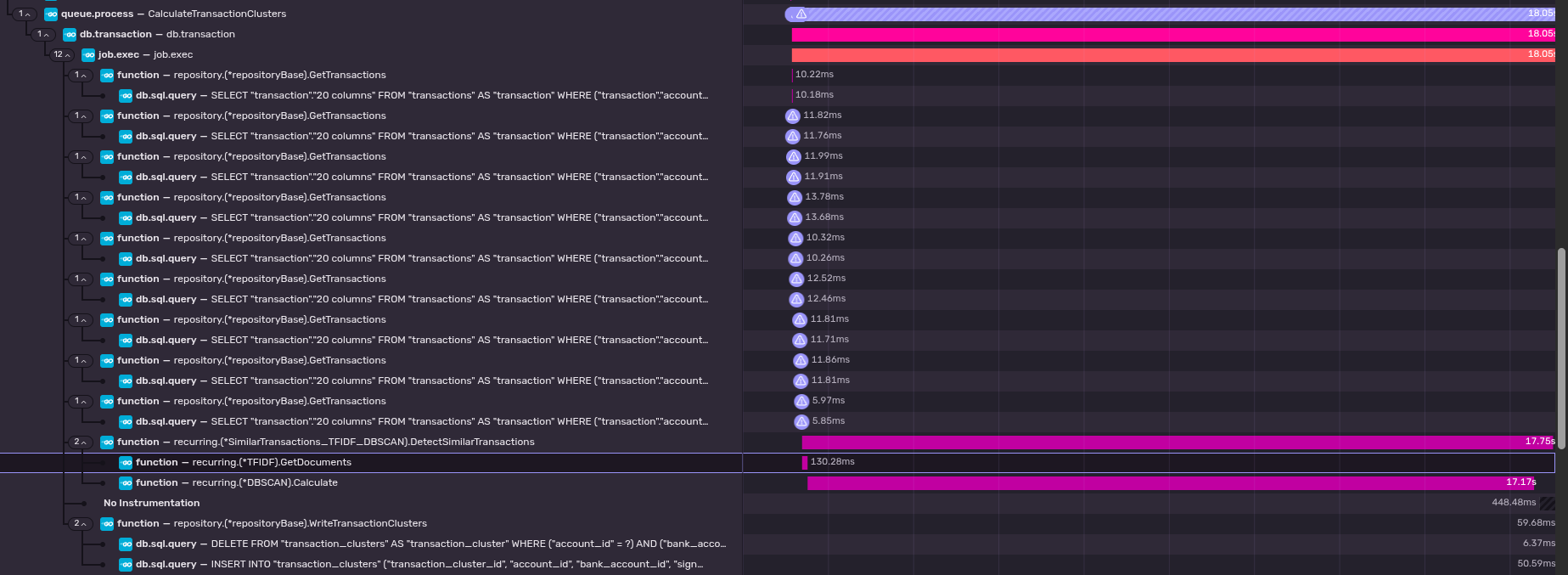As you can see, even the inefficient N+1 query and the tf-idf code is just insignificant compared to the time it takes to perform the DBSCAN. (Note: monetr’s production servers are not using AVX512)

There are surely more ways that I can improve this process, but these are the two that are front of mind for me at the moment. I am not a mathematics expert by any means either so its very possible that the calculations or my implementation of them is not correct. If you would be interested in correcting me and helping me learn more, please let me know. monetr is built in the open and the code is fully available to everyone. I’m here making stupid choices in public so people can point them out sooner.